In Data Science or Data Engineering you constantly hear term “data pipeline”. But there are so many meanings to this term and people often are refering to very specific tools or packages depending on their own background/needs. There are pipelines for pretty much everything and in Python alone I can think of Luigi, Airflow, scikit-learn pipelines, and Pandas pipes just off the top of my head - this article does a good job of helping you understand what is out there.
It can be quite confusing especially if you want a simple and agnostic pipeline that you can customize for your specific needs with no bells and whistles or lock-ins to libraries etc. That is where PyDuct comes in. It is for the simple data engineer who just wants to get stuff done in an ordered and repeatable way.
PyDuct is a simple data pipeline that automates a chain of transformations performed on some data.
PyDuct data pipelines are a great way of introducing automation, reproducibility, structure, and flow to your data engineering projects.
PyDuct was made by Robert Johnson and Alexander Kozlov and Mohammadreza Khanarmuei
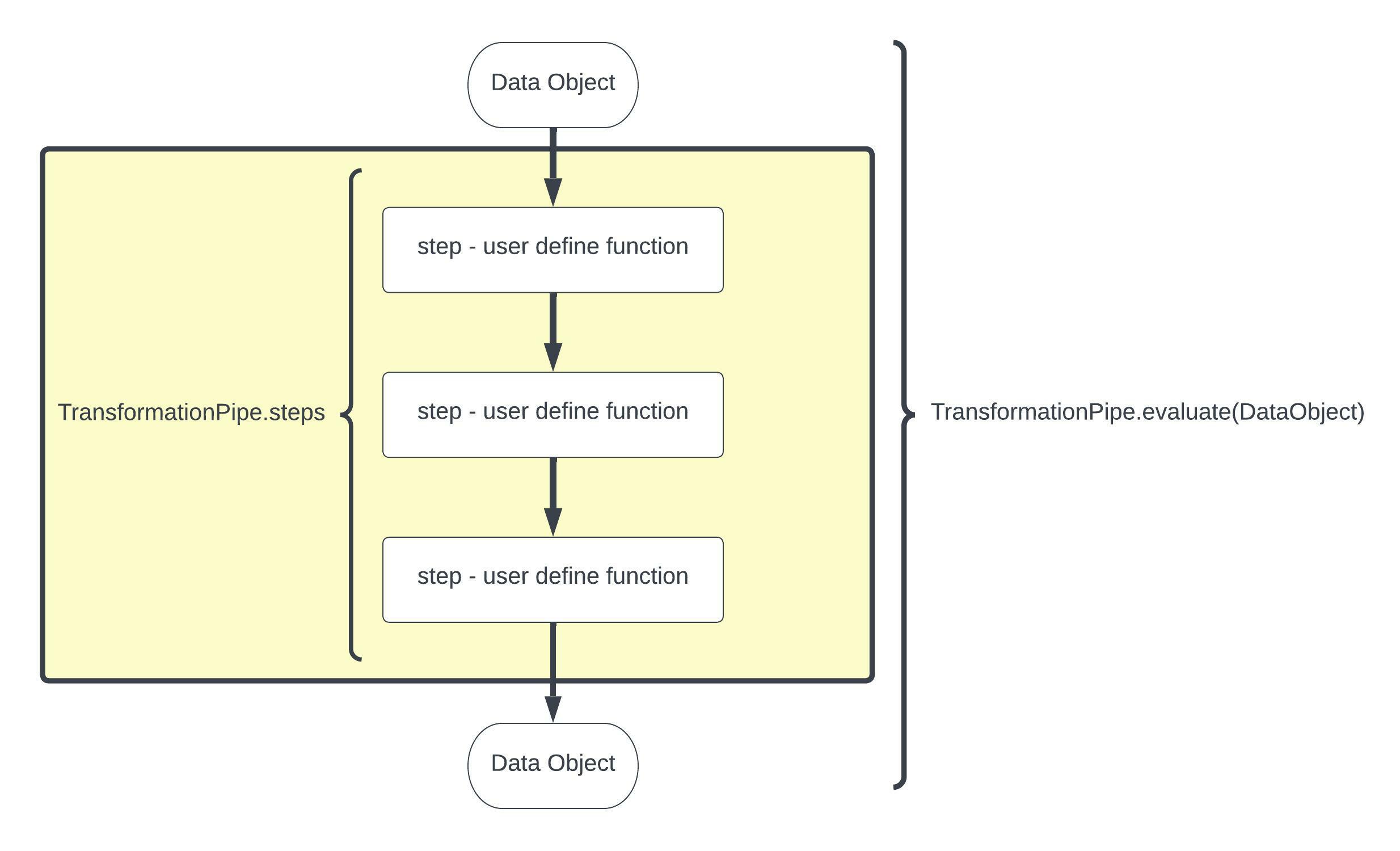
The PyDuct transformation pipelines use user defined transformation functions linked together into a TransformationPipe. The key feature of PyDuct is that the datasource passed in can be almost anything that you desire - e.g. a pandas dataframe, a geopandas dataframe, and iris datacube, a numppy array, so long as your transformation steps read and write the same object PyDuct will work for you.
pip install pyduct
The TransformationPipe class accepts a list of transformation functions,'steps', to be applied sequentially. Each step contains a name and a function, applied to the input DataObject and will return a transformed DataObject. There is also a third argument in a step that is an optional dictionary of parameters to be passed to your step transformation functions.
In order to use PyDuct you need two things - a DataObject and a set of transformation steps
In this very simplified example we will use a geopandas.GeoDataFrame as our input DataObject. To do this we will load an example data set from Kaggle on the global distribution of Volcano Eruptions: https://www.kaggle.com/datasets/texasdave/volcano-eruptions that we have stored in the repo for this package as 'volcano_data_2010.csv'
import pandas
import geopandas
Load the data and put it into a geopandas dataframe:
df1 = pandas.read_csv('../test_data/volcano_data_2010.csv')
# Keep only relevant columns
df = df1.loc[:, ("Year", "Name", "Country", "Latitude", "Longitude", "Type")]
# Create point geometries
geometry = geopandas.points_from_xy(df.Longitude, df.Latitude)
geo_df = geopandas.GeoDataFrame(df[['Year','Name','Country', 'Latitude', 'Longitude', 'Type']], geometry=geometry)
geo_df.head()
Just as an example of something to do we will define only one transformation steps to spatially subset to the Australian region. Yes, i know that this is an unrealistic example but it is just here to show you how to implement pipelines.
We must now write our transformation function - keep in mind that the function must take our DataObject as an input and return a transformed DataObject as a return... in this example that is a geopandas.GeoDataFrame
from pyproj import crs
from shapely.geometry import Polygon, MultiPolygon, box, Point
def spatialCrop(gdf: geopandas.GeoDataFrame, **kwargs):
    """
    This function will apply a sptial limit to a GeoDataFrame based on user-defined limits.
    ----------
    parameters:
        gdf (geopandas.GeoDataFrame): an input GeoDataFrame
        kwargs (dict): parameters,
            - boundingBox (list): an iterable (lon_min, lat_min, lon_max, lat_max) of the specified region.
    Output:
        transformed_gdf (gdp.GeoDataFrame): GeoDataFrame that is spatially limited to the boundingBox.
    """
    if "boundingBox" not in kwargs:
        return gdf

    boundingBox = kwargs["boundingBox"]
    # just an example so we are doing naughty things with the CRS... look away here...
    coord_system = crs.crs.CRS('WGS 84')

    bounding = geopandas.GeoDataFrame(
        {
            'limit': ['bounding box'],
            'geometry': [
                box(boundingBox[0], boundingBox[1], boundingBox[2],
                    boundingBox[3])
            ]
        },
        crs=coord_system)
    limited_gdf = geopandas.tools.sjoin(gdf,
                                        bounding,
                                        op='intersects',
                                        how='left')
    limited_gdf = limited_gdf[limited_gdf['limit'] == 'bounding box']
    limited_gdf = limited_gdf.drop(columns=['index_right', 'limit'])

    return limited_gdf
pipe = TransformationPipe(steps=[
    ('refine region', spatialCrop, {"boundingBox": [80, -50, 180, 0]})
])
geo_df
transformed_geo_df = pipe.evaluate(geo_df)
transformed_geo_df
The power of this work is in its reproducibility and scalablilty.
- Logo art from "Vecteezy.com"
- Demo data from "Kaggle.com"